Blog
Short posts, experiment notes and thoughts from the lab.
Listening To A Stadium From Outside, What Does EEG Measure?
Our brains hold around 86 billion neurons, and EEG can't hear any single one of them. So what are we actually recording?
Our brains hold around 86 billion neurons. Imagine standing outside a football stadium. There are tens of thousands of people inside. You can’t make out what any one person is saying. But when a goal goes in, or a whole stand starts chanting at once, you hear a clear roar even from the street.
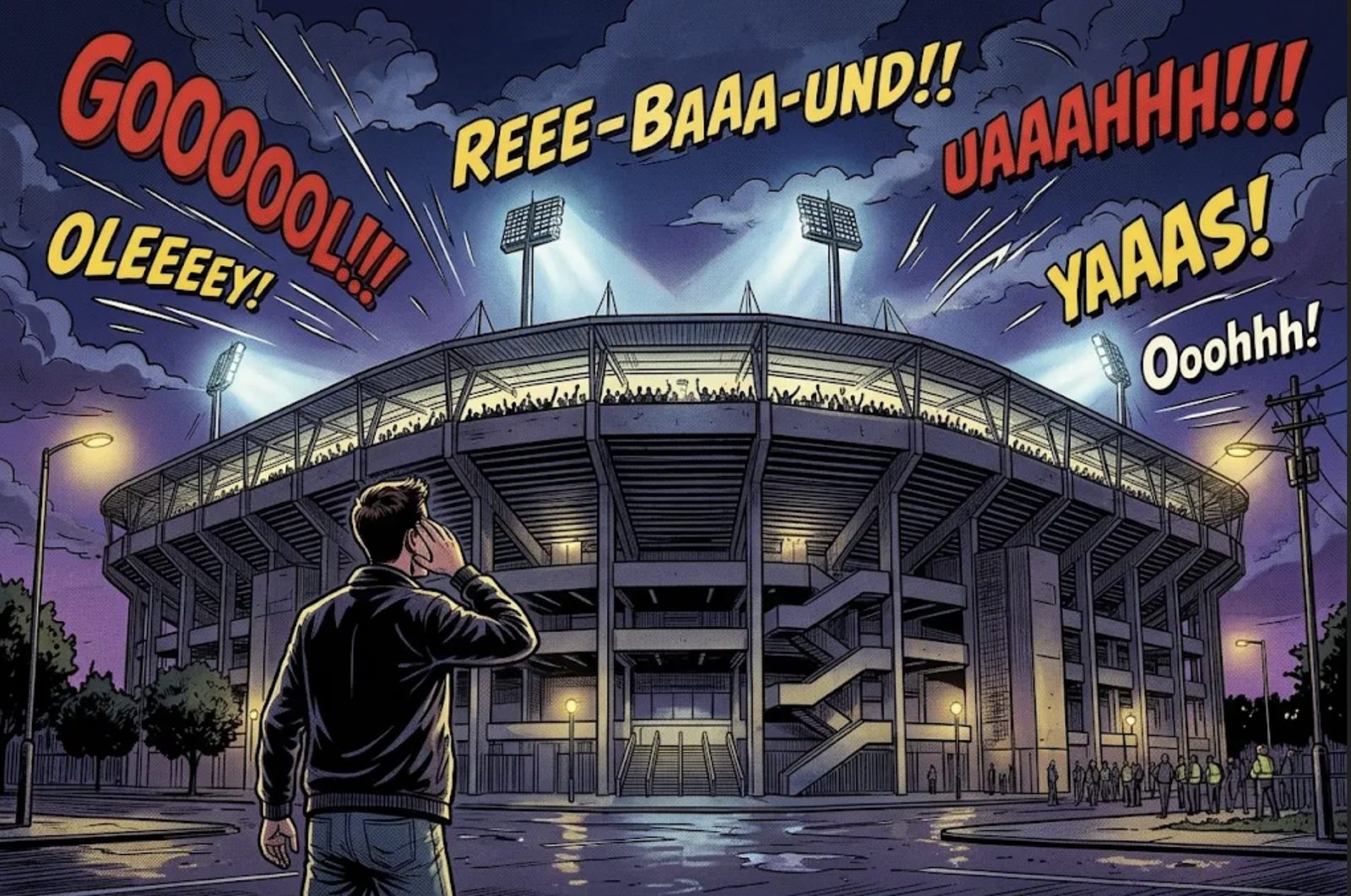
From outside we don't hear individual voices, only the combined roar of the crowd. EEG works exactly like that. Neurons in the brain talk to each other with tiny electrical signals. A single neuron’s signal is far too weak to measure from outside the skull. But when thousands of neurons fire together, in the same rhythm, the combined signal reaches the electrodes we place on the scalp. The waves we see in EEG are the brain’s “collective chants”.
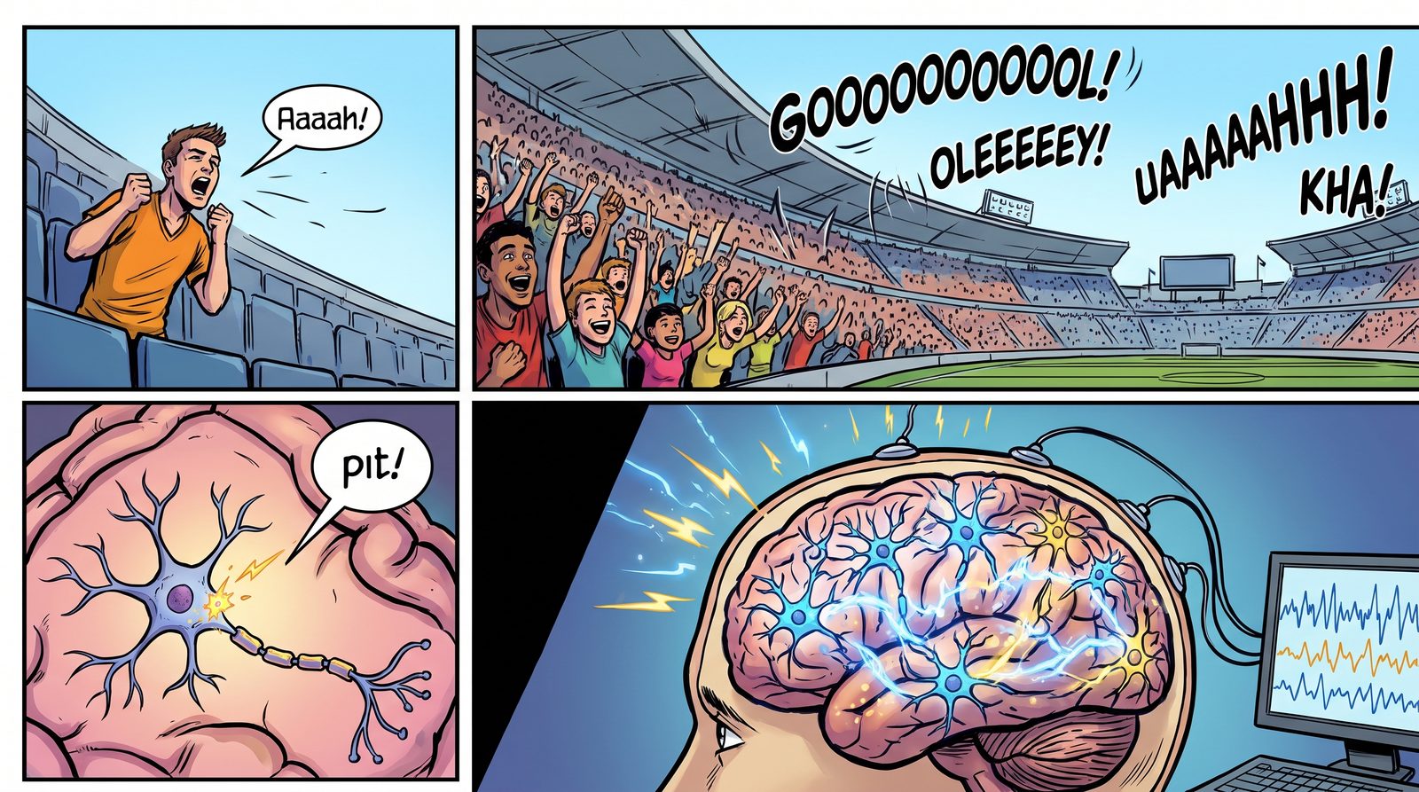
Like a single fan's voice, a single neuron's signal gets lost. When thousands work together, a signal strong enough to reach the electrodes emerges. Rhythms
This collective activity tends to oscillate at certain speeds. We call them frequency bands:
- Delta (0.5–4 Hz): the slow waves of deep sleep.
- Theta (4–8 Hz): drifting off, daydreaming, some memory processes.
- Alpha (8–13 Hz): grows when you close your eyes and relax. It’s the easiest rhythm to see.
- Beta (13–30 Hz): awake, focused, thinking.
- Gamma (30 Hz and above): linked to intense moments when information is being pulled together.
These aren’t “states” with sharp borders. The brain produces a mix of these rhythms all the time, and we look at which ones dominate and by how much.
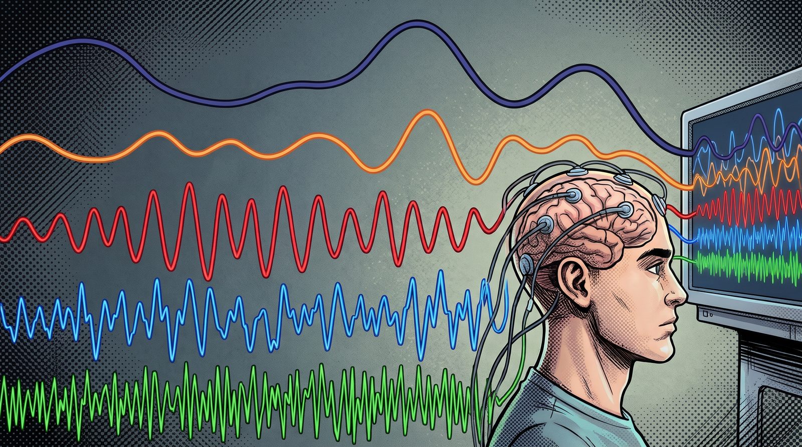
From top to bottom, slow to fast: the EEG signal is a mix of rhythms at different speeds. Strengths And Weaknesses
EEG’s biggest strength is speed. It captures the brain’s response to a stimulus at the millisecond scale. We can measure the gap between the moment you see a logo and the moment your brain reacts to it.
Its weakness is location. Back to the stadium: you can roughly tell which stand the roar comes from, but not which seat. Pinpointing what happens deep inside the brain takes other methods, such as fMRI.
Fast, portable, relatively cheap and completely harmless, EEG is ideal for studying everyday decisions.
References
- Azevedo, F. A. C. et al. (2009). Equal numbers of neuronal and nonneuronal cells make the human brain an isometrically scaled-up primate brain. Journal of Comparative Neurology, 513(5), 532–541. DOI: 10.1002/cne.21974
What Happens In Our Brain The Moment We Trust A Brand?
How do we choose the brands we trust with our money, our data, our health? We are trying to understand what happens in the brain at the moment of a trust decision, without imposing any labels on it.
From Berkay İlber Tunakan’s master’s thesis, supervised by Prof. Dr. Aydın Akan. The study is ongoing; see our research page for details.
You download a new banking app. A company you have never heard of promises you a high interest rate. On the other side is the bank you have used for years, one you may not even like, but that is “at least familiar”. Which one do you trust with your money?
Most of us answer within seconds. But in those few seconds, the brain runs an incredibly complex calculation: Will this brand keep its promise? What if I lose? Has it let me down before? What is my gut telling me?
The Classic Way To Measure Trust: The Investment Game
Economists and neuroscientists have long used a simple but powerful game to measure trust. In the investment game, one player is given money and asked to send part of it to another player. The money sent is multiplied, and the other player decides how much to send back. How much you send is a measure of how much you trust the other person [1].
Studies with this game have produced striking results. In one study, participants given oxytocin, the so-called “bonding hormone”, via nasal spray sent noticeably more money to the other player [2]. It was a vivid sign that trust is not just a rational decision: the body and the brain’s chemistry are involved too.
Trust Is Not In One Place In The Brain
Brain imaging studies show that there is no single “trust centre”. Regions that compute expected reward, structures that evaluate risk and threat, and frontal regions that weigh the decision all work together [3]. EEG studies likewise find trust-related activity spread across different regions of the head [4].
When brands enter the picture, things get even more complex. Recognising a brand, liking it and trusting it are not the same. Trust in a familiar brand and trust in a brand we have just met may be processed by different routes in the brain. A known reputation is even known to change how much attention a person pays to new information [3].
Not Imposing Labels On The Brain
Most EEG studies of trust start with a label: each moment is marked “trusted” or “did not trust”, and an AI model tries to predict that label from the brain signal. The problem with this approach is that it squeezes expectation, risk, remembered experience and felt closeness into a single word.
We turn the question around. Instead of telling the brain “this is trust”, we ask it: How do EEG patterns recorded at moments of trust decisions group together by their similarity to one another? For this we use a kind of AI called unsupervised learning. These methods find the natural groups in the data on their own, without being told the right answer. It is like sorting a box of mixed buttons by colour, size and number of holes without anyone telling you how.
Once these groups emerge, the really interesting part begins: Do the clusters the brain forms on its own match the brand’s familiarity, whether it is liked, the participant’s decision, or the outcome of that decision?
How We Work
Our participants play an investment game featuring well-known brands from different sectors. In each round they decide whether to invest in a brand and see the outcome. Some brands live up to the trust placed in them, while others disappoint over time. This lets us observe trust being built, maintained and broken within the same experiment.
Throughout the game we record EEG and match every decision moment to the brain signal with millisecond precision using an experiment interface we developed ourselves. Participants also fill in a questionnaire measuring how much they trust the brands.
Why It Matters
Trust is the invisible currency of the economy. It underlies many of our decisions, from which bank we use and which medicine we take to which app we trust with our data. Understanding how trust is built and broken in the brain can help brands build a more honest relationship with consumers, and help us understand our own decisions better.
We will write about the results here when we are ready to share them.
References
- Berg, J., Dickhaut, J., McCabe, K. (1995). Trust, reciprocity, and social history. Games and Economic Behavior, 10(1), 122–142. doi:10.1006/game.1995.1027
- Kosfeld, M., Heinrichs, M., Zak, P. J., Fischbacher, U., Fehr, E. (2005). Oxytocin increases trust in humans. Nature, 435, 673–676. doi:10.1038/nature03701
- Riedl, R., Javor, A. (2012). The biology of trust: Integrating evidence from genetics, endocrinology, and functional brain imaging. Journal of Neuroscience, Psychology, and Economics, 5(2), 63–91. doi:10.1037/a0026318
- Wang, M. et al. (2018). EEG-based neural correlates of trust in human-autonomy interaction. IEEE Symposium Series on Computational Intelligence (SSCI), 350–357. doi:10.1109/SSCI.2018.8628649
A Colourful Map Of A Scent In The Brain
What happens in our brain the moment we smell something? We turned the EEG recordings of 57 participants into colourful heatmaps and showed them to an AI. The result was a model that told scented and unscented moments apart almost without error.
Study presented at TIPTEKNO 2025 by Dr. Faezeh Yeganli, Prof. Dr. Aydın Akan and Dr. Rıza Sadıkzade: “Olfactory Emotion Recognition Using EEG Spectral Topographic Heatmaps and CNNs” (doi:10.1109/TIPTEKNO68206.2025.11270101).
The faint scent of vanilla that greets you when you walk into a shop is no accident. From airport terminals to cosmetics counters, scents are chosen deliberately to influence how we feel and what we do. But how do we measure what a scent really makes us feel? Asking “Did you like it?” tells only part of the story.
In our smell post we explained why smell reaches the brain by a shortcut. In this post we explain how we “photographed” the trace that shortcut leaves in the brain.
Reading The Brain Like A Weather Map
EEG records brain activity from electrodes on the scalp with millisecond resolution. But a raw EEG recording is just dozens of wiggly lines side by side. To the human eye, it is hard to make sense of.
In this study we took a different route: we turned EEG into a weather map. Brain signals are not one rhythm but waves oscillating at different speeds: slow delta and theta, faster alpha, beta and gamma. We calculated how strong each rhythm was over each region of the head and placed it in colour on a map of the head seen from above. Red regions show where that rhythm is strong, blue where it is weak.
Each one-second slice of EEG thus became a picture that can be read at a glance. And there is a type of AI that is very good at looking at pictures.
An AI That Looks At Pictures
Convolutional neural networks (CNNs) were developed to recognise faces or objects in photographs. We explained how they work in our CNN post. We showed such a network hundreds of heatmaps from scented and unscented moments and taught it to tell the two apart.
Fifty-seven participants took part. Each was recorded with EEG in both a scented and an unscented condition, and after each condition they rated how aroused (calm to excited) and how pleased they felt. The model learned to classify these two dimensions separately.
We made an important choice here: we kept the model small and simple. In earlier work we had extracted many time, frequency and nonlinear features from the EEG (TIPTEKNO 2024). This time we built a lightweight model that relies only on frequency information and the map of a single rhythm. The aim was a method simple enough to run one day in real-time, portable systems.
Theta Waves Give The Scent Away
The results surprised us too:
- For arousal, theta waves gave the best result: the model told scented and unscented moments apart with 98.4% accuracy, getting only one of the test samples wrong.
- For pleasure, theta and beta waves gave the best result at 96.6% accuracy.
- Delta and gamma waves carried less information.
The heatmaps show why: in scented moments, theta activity concentrates clearly over the frontal and temporal regions, roughly beneath the forehead and temples. In unscented moments it is weaker and more diffuse. These regions are closely connected to the limbic structures involved in emotion and memory. Given theta’s link to attention and emotional memory, it makes sense to see the EEG trace of smell’s “shortcut” exactly here.
Our lightweight model also outperformed better-known networks such as MobileNetV2 and SqueezeNet on the same data.
Why It Matters
Being able to read what a scent makes us feel directly from brain signals, without asking, opens many doors. Measuring more objectively how a perfume, a product or a store environment affects consumers is only one of them. The simplicity of the method also makes it easier to bring to real-time applications and brain–computer interfaces. Our next step is to test the model on participants it has never seen and to take the changes in the signals over time into account.
How Does Aircraft Noise Affect Our Attention And Our Heart?
For people living near airports, aircraft noise is part of daily life. In this capstone project we recorded the brain activity and heart rate of participants solving an attention test under different noise levels.
Undergraduate capstone project (FENG 497/498) by Berkay İlber Tunakan, Altuğ Güneş, Duygu Köybaşı and Can Mungan, supervised by Prof. Dr. Aydın Akan.
Imagine living near an airport. Every few minutes, whether you open a window, take a phone call or try to concentrate, the sound of an aircraft cuts in. Noise pollution is one of the most widespread environmental problems in big cities today, and aircraft noise is among its most intense forms. It can disrupt sleep, raise stress and threaten hearing. But how does it affect our attention and mental workload?
Noise In The Courtroom: The Osaka Airport Case
Lawsuits in Japan show most strikingly that aircraft noise is more than a nuisance. In 1969, residents living directly under the take-off and landing routes of Osaka International Airport (Itami) sued the state, arguing that aircraft noise and vibration were harming their daily lives and health. They asked for flights to be stopped between 9 p.m. and 7 a.m. and for compensation for past and future damages.

Osaka International Airport (Itami) and the housing that reaches right up to the runway, 1985. Source: National Land Image Information (Color Aerial Photographs), Ministry of Land, Infrastructure, Transport and Tourism of Japan, via Wikimedia Commons. In 1975 the Osaka High Court recognised the harm to the residents’ health and ordered night flights to be halted during those hours. When the case reached Japan’s Supreme Court in 1981, the night-flight injunction was rejected, but compensation for past damages was upheld (English summary of the Supreme Court judgment). In Japan this case paved the way for a series of noise lawsuits around military bases that continue to this day:
- Yokota (Tokyo): In 2007 the Supreme Court ordered compensation for past damages to about 6,000 plaintiffs but rejected the demand to halt night flights (The Japan Times).
- Atsugi (Kanagawa): In 2014 the Yokohama District Court became the first district court to order night flights by Self-Defense Forces aircraft to be suspended, and the Tokyo High Court upheld the decision in 2015 (The Japan Times).
- Kadena (Okinawa): In 2017 about 22,000 residents were awarded ¥30.2 billion, the largest noise damages in Japanese history (The Japan Times). The lawsuits were still continuing in 2026 (Stars and Stripes).
These cases show that the impact of aircraft noise on quality of life is recognised even in law. Yet studies examining how this impact shows up in the brain and body with objective measurements are still limited. That is where our project started.
How We Measured It
Thirty healthy participants aged 20 to 30 solved an n-back test, which measures attention and working memory. We used the two-step (2-back) version: letters appear on the screen one at a time, and the participant presses a button when the current letter matches the one shown two letters earlier. The test was repeated under three sound conditions: silence, moderate aircraft noise and loud aircraft noise.
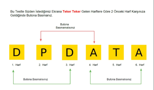
Instructions shown to participants (in Turkish): press the button when the letter matches the one two letters earlier. 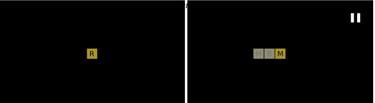
Example screens during the test: letters appear one at a time. During the test we recorded brain activity with our lab’s EEG system and heart rate with a wrist-worn photoplethysmography (PPG) band. We filtered the EEG signals and extracted time- and frequency-domain features for each sound condition. We then trained machine learning models that predict the participant’s test performance from these features.
What We Found
Louder sound, faster heart. As sound level and the mental load of the test increased, participants’ heart rate rose. The increase was clear in about 80% of male participants and about 60% of female participants.
Noise did not hurt performance as much as expected. Our initial expectation was that more noise would mean less attention and more errors. The results were not that simple. The number of correct responses was similar across all three conditions and decreased only slightly as noise increased. Errors were highest in silence, which may partly be because silence was the participants’ first round of the test. Under moderate and loud noise, errors dropped markedly. This suggests that a certain level of background sound may help keep attention alert.
EEG helped predict performance. A voting classifier combining support vector machines, random forest and gradient boosting predicted participants’ test performance from EEG with about 70% accuracy. On the central Cz channel this model reached the highest AUC, 0.81.
Conclusion
Aircraft noise leaves an immediate trace in the body: the heart speeds up, and this response differs between people and even between sexes. Its effect on attention is more complex than we thought. In a short test, noise did not impair performance, and moderate noise even reduced errors. These findings show the value of assessing the effects of noise not only through test scores but together with brain and body signals.
This project was one of the first steps towards the EEG and multimodal biosignal work our lab carries out today.
3Blue1Brown, The Essence Of Linear Algebra And Calculus
For those who want to see the picture before starting long courses: two short video series that explain linear algebra and calculus through animation.
Two series from the 3Blue1Brown channel explain the foundations of maths through visual intuition before formulas: Essence of Linear Algebra and Essence of Calculus.
What’s in it? The linear algebra series covers vectors, matrices as linear transformations, the determinant, the dot product, change of basis, and eigenvectors and eigenvalues. The calculus series covers what a derivative is, the chain rule, Euler’s number e, limits, integration and the fundamental theorem of calculus, and Taylor series.
Why we recommend it: Made up of 10 to 20-minute videos, these series are ideal to watch before, or alongside, Strang’s linear algebra course or MIT’s calculus courses. The view of “a matrix as a transformation” in particular makes many signal processing concepts click into place at once.
Who is it for? High-school maths is enough. Anyone who has met these topics before but never quite settled the “why”.
- Series pages: Essence of Linear Algebra and Essence of Calculus
MIT 6.041, Probability With John Tsitsiklis
The probability foundation everyone working with noisy signals and uncertain results needs, in one of its clearest presentations.
MIT 6.041 Probabilistic Systems Analysis and Applied Probability is a probability course taught at MIT by Prof. John Tsitsiklis. Lecture videos, slides, problem sets and exams are free on MIT OpenCourseWare.
What’s in it? Probability models, conditional probability and Bayes’ rule, discrete and continuous random variables, covariance, Bernoulli and Poisson processes, Markov chains, the law of large numbers, the central limit theorem, and Bayesian and classical statistical inference.
Why we recommend it: EEG is a noisy signal, participants differ from one another and every classification result is a probability. Deciding whether a result is meaningful, understanding why a model got something wrong or seeing the assumptions behind machine learning methods all require a solid foundation in probability. Tsitsiklis teaches it in an orderly and exceptionally clear way.
Who is it for? Anyone who knows calculus and wants a solid introduction to probability.
- Course page: MIT OCW, 6.041
Stanford EE263, Linear Dynamical Systems With Stephen Boyd
From linear algebra to state-space models: a widely referenced Stanford course that teaches linear system theory through engineering examples.
Stanford EE263 Introduction to Linear Dynamical Systems is a course taught at Stanford by Prof. Stephen Boyd. The lecture videos, notes, assignments and exams are free on Stanford Engineering Everywhere.
What’s in it? Applied linear algebra, least-squares and least-norm solutions, state-space models, the matrix exponential, stability analysis through eigenvalues, the singular value decomposition, controllability and observability.
Why we recommend it: Where Oppenheim’s course describes systems through their input and output signals, Boyd’s looks “inside” the same systems: state variables and matrices. With examples from circuits, signal processing, communications and control, it shows the full engineering power of the idea in our linearity post. Boyd’s energetic, witty delivery is a bonus.
Who is it for? Engineering students with basic linear algebra. A background in control or signals isn’t required, but makes the course more enjoyable.
- Course page: Stanford Engineering Everywhere, EE263
MIT 18.01 And 18.02, Single And Multivariable Calculus
From derivatives to integrals, from gradients to multiple integrals: two calculus courses built from start to finish for independent learners.
MIT’s two core calculus courses are published for free in the OCW Scholar format designed for independent learners: Prof. David Jerison’s 18.01SC Single Variable Calculus and Prof. Denis Auroux’s 18.02SC Multivariable Calculus.
What’s in it? 18.01 covers limits, derivatives and their applications, integration, the fundamental theorem of calculus and infinite series. 18.02 covers vectors and matrices, partial derivatives, gradients, multiple integrals and vector calculus. Alongside the lecture videos there are problem-solving videos, worked examples and exams.
Why we recommend it: Calculus sits underneath almost every topic on this site. The Fourier transform is an integral, signal filters are defined by differential equations, and a neural network learns by following the gradient of its error. The partial derivative and gradient units in 18.02 are exactly what you need to understand what “gradient descent” in machine learning actually does.
Who is it for? High-school algebra and trigonometry are enough for 18.01. 18.02 follows on from 18.01.
- Course pages: MIT OCW, 18.01SC and MIT OCW, 18.02SC
MIT 18.06, Linear Algebra With Gilbert Strang
Possibly the most watched maths course on the internet. The classic that engineers have turned to for years to understand linear algebra intuitively.
MIT 18.06 Linear Algebra, taught at MIT by Prof. Gilbert Strang, is one of the most watched maths courses in the world. Videos, problem sets and exams with solutions are free on MIT OpenCourseWare.
What’s in it? Systems of linear equations, matrices, vector spaces, orthogonality and least squares, determinants, eigenvalues and eigenvectors, and the singular value decomposition (SVD).
Why we recommend it: Linear algebra is the language of biosignal processing and machine learning. A multichannel EEG recording is a matrix; cleaning artefacts with ICA, reducing dimensions with PCA or training a neural network are all matrix operations. Strang builds these ideas through their meaning before their formulas. The “Fourier of a graph” in our graph theory post is really an eigenvector story too.
Who is it for? Anyone with high-school maths. The videos were recorded in 1999, but the teaching hasn’t aged a day.
- Course page: MIT OCW, 18.06 Linear Algebra
Copenhagen Business School, An Introduction To Consumer Neuroscience
Perhaps the best-known online introduction to neuromarketing. From attention to emotion, memory to decision making, ethics included.
An Introduction to Consumer Neuroscience & Neuromarketing is an introductory course on Coursera taught by Thomas Zoëga Ramsøy of Copenhagen Business School. The course content can be followed for free on Coursera, with a paid option for those who want a certificate.
What’s in it? What neuromarketing is and which methods it uses, attention and consciousness, sensory marketing, emotions, wanting and liking, learning and memory, decision making and the ethics of neuromarketing. There are also interviews with guests from industry and academia.
Why we recommend it: It draws a broad map of the idea of “listening to what surveys can’t tell you” that we described in our neuromarketing post. The distinction between wanting and liking, and the ethics module in particular, are topics anyone who wants to work in this field should know.
Who is it for? No background needed. Anyone curious about consumer behaviour, whether from marketing, psychology or engineering.
Neuromatch Academy, Computational Neuroscience
A fully open computational neuroscience curriculum built by researchers from all over the world. Learn by doing, with Python notebooks.
Neuromatch Academy is an online school run by volunteer researchers, set up to make computational neuroscience accessible to everyone. All its course materials are published for free as an open coursebook and can be reused freely.
What’s in it? Model building basics, statistical inference, linear systems, machine learning for neural data, dimensionality reduction, decision making, dynamical systems and networks. Each topic comes with short videos and Python notebooks that run in the browser.
Why we recommend it: It’s one of the best answers to what the “computational neuroscience” in our lab’s name actually means. It teaches by having you write code, not by having you listen. A good place to see how the signal processing and AI posts on this site meet neuroscience.
Who is it for? Students and researchers with basic Python and some maths who want to approach neuroscience from the computational side.
- Coursebook: Neuromatch Academy, Computational Neuroscience
3Blue1Brown, Seeing Neural Networks
A short video series that explains how neural networks learn through animation rather than formulas. Possibly the best place to start.
3Blue1Brown is Grant Sanderson’s much-loved YouTube channel that explains maths through animation. Its neural networks series explains, in a handful of short videos, what a neural network is and how it learns.
What’s in it? Neurons and layers, gradient descent, backpropagation and, in later chapters, the Transformer and attention behind large language models.
Why we recommend it: It isn’t a university course, but it may be the best starting point. It shows the picture before the formulas, so when you later move on to courses like CS229 or CS231n you know what you’re looking for. If you’ve read our Transformer post, the chapters on attention are a nice follow-up.
Who is it for? High-school maths is enough. Everyone, including people who know nothing about AI.
- Series page: 3Blue1Brown, Neural Networks
Stanford CS231n, Deep Learning For Images
The course everyone who wants to learn convolutional neural networks runs into sooner or later. Notes, slides and assignments are free.
Stanford CS231n Deep Learning for Computer Vision is a graduate course taught at Stanford by Fei-Fei Li and her team. Lecture notes, slides and assignments are free at cs231n.stanford.edu, and the videos of a recent term have been published on Stanford Online’s YouTube channel.
What’s in it? Image classification, training neural networks, convolutional networks and their architectures, sequence models and attention, generative models, object detection and segmentation.
Why we recommend it: Although its name says “vision”, the course builds the foundations of deep learning very solidly. The lecture notes in particular are one of the clearest explanations of the convolution we described with a torch in our CNN post. It’s also a good basis for work that turns EEG into topographic maps and classifies them with CNNs.
Who is it for? Anyone with Python and basic linear algebra who wants to learn deep learning through hands-on assignments.
- Course page: Stanford CS231n
Stanford CS229, Machine Learning With Andrew Ng
Perhaps the best-known university course on machine learning. Derivations on the blackboard, free videos and lecture notes.
Stanford CS229 Machine Learning, taught at Stanford by Andrew Ng, is one of the best-known courses in the field. The 2018 lecture videos are on Stanford Online’s YouTube channel, and the lecture notes and problem sets are free at cs229.stanford.edu.
What’s in it? Linear and logistic regression, support vector machines, decision trees and ensemble methods, neural networks, model selection and cross-validation, independent component analysis (ICA) and reinforcement learning.
Why we recommend it: The maths behind the methods whose intuition we covered in our SVM, Random Forest and XGBoost posts is derived here step by step. There’s also a lecture on ICA, which we use to clean artefacts from EEG.
Who is it for? Anyone with probability, linear algebra and calculus who wants machine learning to stop being a black box. It’s a maths-heavy course.
- Course page: Stanford CS229
Stanford EE261, The Fourier Transform With Brad Osgood
A whole term devoted to the Fourier transform: Stanford's 30-lecture series, free together with notes and exams.
Stanford EE261 The Fourier Transform and its Applications is an undergraduate course taught at Stanford by Prof. Brad Osgood. It is published for free on Stanford Engineering Everywhere with videos, course notes, assignments and exams.
What’s in it? Fourier series, the Fourier transform and its properties, convolution, sampling, the discrete Fourier transform and FFT, linear systems and the higher-dimensional Fourier transform. Thirty lectures in all.
Why we recommend it: Where Oppenheim’s course builds the general framework of signal processing, Osgood’s devotes a whole term to a single tool, the Fourier transform. With his witty delivery and physical examples, it’s ideal for anyone who wants to anchor the ideas in our Fourier post in solid maths. The course notes were later published as a book.
Who is it for? Anyone with calculus and basic linear algebra who wants to learn Fourier analysis in depth.
- Course page: Stanford Engineering Everywhere, EE261
MIT 9.13, The Human Brain With Nancy Kanwisher
From face recognition to language, from music to attention: an enjoyable undergraduate course on how the brain works, with no background required.
MIT 9.13 The Human Brain is an undergraduate course taught by Prof. Nancy Kanwisher, one of the leading figures in cognitive neuroscience. The lecture videos and notes are published for free on MIT OpenCourseWare.
What’s in it? Methods for studying the brain, face and scene perception, navigation, number, hearing and speech, music, language, understanding other minds, brain networks, and attention and awareness.
Why we recommend it: Kanwisher argues that the questions in this field are ones anyone can ask with no background at all, and the course is taught in that spirit, through real stories and experiments. It’s a good starting point for anyone curious about which part of the brain does what, and how we measure it. If you’ve read our EEG and fNIRS posts, you’ll also see where those methods sit in the bigger picture.
Who is it for? Anyone curious about neuroscience, whether they come from engineering or psychology.
- Course page: MIT OCW, 9.13 The Human Brain
MIT 6.S191, A Fast Introduction To Deep Learning
A short, intensive deep learning course rewritten every year. Videos, slides and browser-based labs are free.
MIT 6.S191 Introduction to Deep Learning is a short, intensive deep learning course held at MIT every year. All the lecture videos, slides and labs are published for free at introtodeeplearning.com.
What’s in it? Neural network fundamentals, sequence models, networks for images, generative models, reinforcement learning and large language models. Each lecture runs about an hour. The labs run on Google Colab, so you don’t need to install anything.
Why we recommend it: The content is refreshed every year, so it keeps up with where the field is. It’s a good follow-up for anyone who wants to see the maths and code behind the ideas in our CNN, LSTM and Transformer posts.
Who is it for? Anyone with a little Python who wants a fast but solid introduction to deep learning. Recordings from previous years are archived on the site too.
- Course page: MIT 6.S191 Introduction to Deep Learning
Signals And Systems With Oppenheim From MIT
A free lecture series, taught in chalk on a blackboard, by the author of the classic signal processing textbook. Everything from Fourier to sampling is here.
Almost everyone who works with signal processing has Oppenheim and Willsky’s Signals and Systems on their shelf. MIT publishes for free on OpenCourseWare the video lecture series that the book’s author, Alan V. Oppenheim, prepared to go with it, under the name RES.6-007 Signals and Systems.
What’s in it? Linear time-invariant systems, convolution, the Fourier series and transform, filtering, modulation, sampling, and the Laplace and z-transforms. Alongside the videos you can download lecture notes, problem sets and their solutions.
Why we recommend it: The recordings were made many years ago and the picture quality isn’t up to today’s standards. But Oppenheim’s way of building each concept from intuition and only then tying it to the maths is still unmatched. It’s a good next step for anyone who has read our linearity, Fourier and sampling posts and wants to go deeper.
Who is it for? Anyone with basic maths and calculus who wants a solid introduction to signal processing.
- Course page: MIT OCW, RES.6-007 Signals and Systems
- Textbook: Oppenheim, A. V., Willsky, A. S. Signals and Systems. Prentice Hall.
Nonlinearity, Adding Ten More Cars To Traffic
Adding ten cars to an empty road changes nothing. Adding ten cars to a busy road can bring traffic to a standstill. The brain often behaves the same way.
In the linearity post we talked about systems where doubling the input doubles the output. Many real-world systems don’t behave like that.
Think of traffic. Add ten cars to an empty road at night and nothing changes. Add ten cars to the same road at rush hour, when it’s already full, and traffic can grind to a halt. The same amount of change has completely different effects depending on the system’s current state. That is what nonlinearity means.
Something similar happens when you turn a speaker all the way up: the sound doesn’t just get louder, it starts to crackle. Nonlinear systems can produce new frequencies that weren’t in the input at all.
Why Isn’t The Brain Linear?
Start with the smallest building block. A neuron stays silent until its incoming signals cross a certain threshold. Once the threshold is crossed, it fires fully, all or nothing. There is no half-firing. That is the exact opposite of linear behaviour. A network of billions of such units wired together shows very rich, and sometimes hard to predict, behaviour.
That’s why studying EEG only with linear tools, for example only the spectrum, can miss part of the picture. As summarised in Stam’s review, nonlinear analysis methods measure a signal’s complexity, regularity and predictability. Entropy measures and fractal dimension are the best known.
In our lab we have compared these two views too: to detect an olfactory stimulus in EEG, we evaluated linear and nonlinear features side by side. More often than not, the best results come from using both together.
References
- Stam, C. J. (2005). Nonlinear dynamical analysis of EEG and MEG: review of an emerging field. Clinical Neurophysiology, 116(10), 2266–2301. doi:10.1016/j.clinph.2005.06.011
- Akbugday, B., Akan, A., Pehlivan, S., Sadighzadeh, R. (2022). An assessment of linear and nonlinear features for detecting olfactory stimulus in EEG. Medical Technologies Congress (TIPTEKNO). doi:10.1109/tiptekno56568.2022.9960190
Linearity, What Happens When You Double The Volume?
Turn a speaker up to twice the volume and the music comes out twice as loud, but the song stays the same. The most powerful tools of signal processing rest on this simple behaviour.
In signal processing, a “system” is anything that takes a signal in and gives a signal out: a filter, an amplifier, even the skull. A system being linear comes down to two simple conditions.
Scaling: Double the input and the output doubles. Turn up a speaker and the song stays the same, it just gets louder.
Adding: Feed two inputs together and the output is the sum of the outputs you’d get from each one separately. If two speakers in a room play different songs, what reaches your ear is the sum of the two.
Together these two conditions are called superposition. A third condition is often added: the system behaves the same today as tomorrow, i.e. it is time-invariant. Systems that meet all three are called LTI (linear, time-invariant) systems.
Why Does It Matter So Much?
Because to understand a linear system you don’t have to test it with every possible input. The Fourier transform splits any signal into a sum of simple sine waves. If you know what the system does to individual sine waves, superposition tells you what it does to any signal. Almost all of filter design rests on this idea.
This is also what makes EEG understandable. As the electrical activity of different sources in the brain passes through the skull and scalp to the electrodes, it adds up in a largely linear way. The signal we see at one electrode is a weighted sum of many sources. The methods we use to separate artefacts such as eye blinks from the signal also rely on this assumption.
But the world isn’t always this tidy. We cover that in the nonlinearity post.
References
- Akan, A., Chaparro, L. F. (2024). Continuous-time systems. Signals and Systems Using MATLAB, Elsevier. doi:10.1016/b978-0-44-315709-7.00012-4
- Akan, A., Chaparro, L. F. (2024). Discrete-time signals and systems. Signals and Systems Using MATLAB, Elsevier. doi:10.1016/b978-0-44-315709-7.00018-5
Sampling, Why Do Wheels Spin Backwards In Films?
In films, the wheels of a fast car sometimes seem to spin backwards. That small illusion explains the most basic rule of digital signal processing.
A brain signal flows continuously. A computer can’t store something continuous, so it takes snapshots of the signal at regular intervals. We call this sampling. If we take 500 snapshots per second, our sampling frequency is 500 Hz.
So how many snapshots per second are enough?
Wheels Spinning Backwards
Remember the wheels of a fast car in a film. Sometimes they seem to slow down, stop, or even spin backwards. The reason is the camera: it takes a fixed number of frames per second. If the wheel makes almost a full turn between two frames, the camera catches it as if it had moved back a little.
The same happens with signals. If you don’t sample a fast-oscillating wave often enough, it shows up in the recording as a slower, fake wave. This is called aliasing. The sneaky part: looking at the recording, you can’t tell anything went wrong.
The Nyquist Rule
The fix rests on a simple rule: you must sample more often than twice the highest frequency in the signal. Shannon set out this limit clearly in 1949. When the rule holds, the original continuous signal can be recovered exactly from its samples.
If we want to see gamma activity reaching up to 100 Hz in EEG, we need to sample at 200 Hz or more. In practice, EEG devices usually run between 250 and 1000 Hz. There is also a safety step: just before sampling, a filter removes frequencies above the limit, so the “backwards wheel” never makes it into the recording.
References
- Shannon, C. E. (1949). Communication in the presence of noise. Proceedings of the IRE, 37(1), 10–21. doi:10.1109/JRPROC.1949.232969
- Akan, A., Chaparro, L. F. (2024). Sampling theory. Signals and Systems Using MATLAB, Elsevier. doi:10.1016/b978-0-44-315709-7.00017-3
The Fourier Transform, Finding The Smoothie's Recipe
If someone handed you a smoothie, could you say how much strawberry and how much banana went into it? The Fourier transform does exactly that for signals.
Think of a glass of smoothie. When you taste it, you get a single flavour. But inside there are strawberries, blueberries, banana and milk in certain proportions. The Fourier transform is the tool that works out this recipe for a signal.
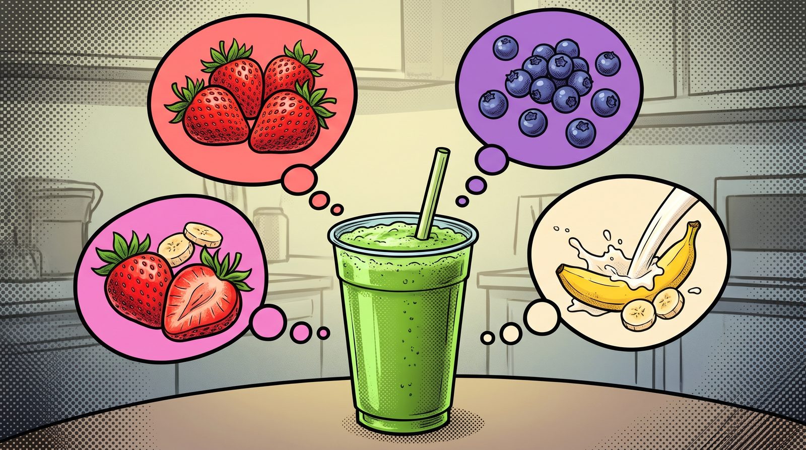
A single flavour, but behind it are several ingredients in certain proportions. Fourier’s idea was this: however complicated it looks, every signal can be written as a sum of simple waves oscillating at different speeds, that is, sine waves. The transform tells us how much of each speed, each frequency, there is. This recipe is called the spectrum.
The key point: the Fourier transform doesn’t change the signal, it just describes it in another language. If you know the recipe, you can make the smoothie again. If you know the spectrum, you can get the signal back exactly.
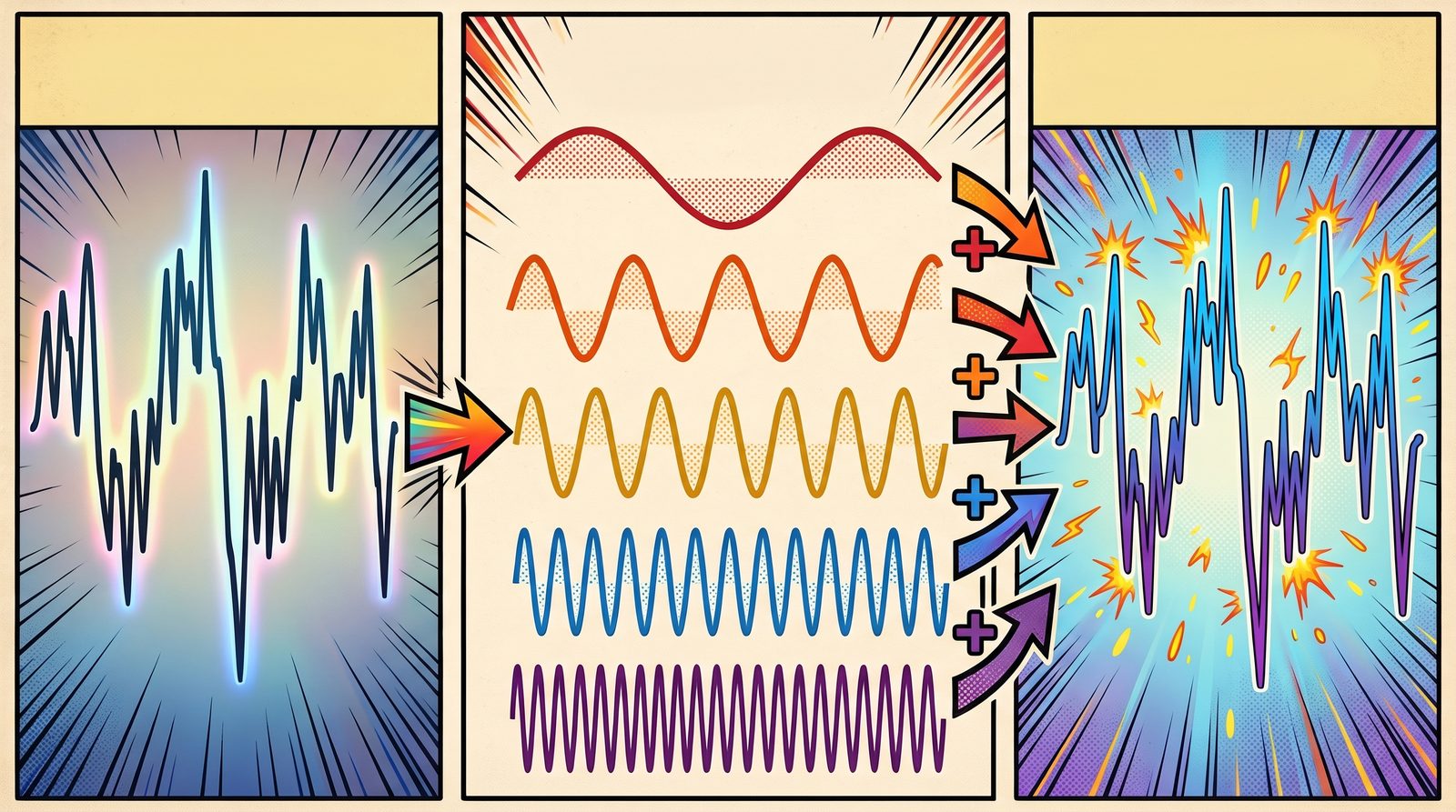
Left: the complex signal. Middle: the sine waves at different speeds that make it up. Right: the signal rebuilt by adding those sine waves together. Why Is It Everywhere?
When we say “alpha power went up” in EEG, we are actually looking at the spectrum: the share of the 8–13 Hz ingredient in the recipe has grown. Many jobs, such as removing noise, separating rhythms or compressing a signal, become much easier once the signal is translated into this language.
What made it practical was the fast Fourier transform (FFT). Computing the recipe of a 1024-sample signal the straightforward way takes about a million operations. The algorithm Cooley and Tukey published in 1965 does the same job in roughly ten thousand. Today it runs everywhere, from the music app on your phone to EEG software.
If you’d like to see the Fourier transform in more detail alongside EEG features, have a look at the spectral features post.
References
- Akan, A., Chaparro, L. F. (2024). Frequency analysis: the Fourier transform. Signals and Systems Using MATLAB, Elsevier. doi:10.1016/b978-0-44-315709-7.00015-x
- Cooley, J. W., Tukey, J. W. (1965). An algorithm for the machine calculation of complex Fourier series. Mathematics of Computation, 19(90), 297–301. doi:10.1090/S0025-5718-1965-0178586-1
Graph CNNs, Neural Networks That Listen To Their Neighbours
A CNN looks at an image with a torch, because pixels sit on a neat grid. But what if the data doesn't sit on a grid, but on a network?
In the CNN post we described how convolutional neural networks examine an image as if sweeping it with a torch. Each time, the torch lights up a small square: a pixel and its neighbours to the left, right, above and below. That works because in an image every pixel’s neighbours are clearly defined, and everyone has the same number of them.
Now think of an EEG cap. The electrodes don’t sit on a neat grid on the head. Some have four electrodes nearby, some only two. And two electrodes sitting side by side on the head doesn’t mean the brain activity under them is linked. Two distant regions may be working closely together. The structure that best describes this kind of data isn’t a grid but a graph: electrodes as nodes, the relationships between them as edges.
Taking Advice From The Neighbours
Graph convolutional networks (GCNs) put the torch away and use a more social method. Picture an apartment building. Every flat has its own opinion. At a meeting, everyone listens only to their next-door neighbours and updates their own opinion by blending it with theirs. Who counts as whose neighbour is set by the building’s floor plan, the graph.
One GCN layer does exactly this:
- Each node gathers the features of its neighbours.
- It combines them with its own feature.
- It transforms the result with learned weights to produce a new feature.
This simple rule, proposed by Kipf and Welling in 2017, became the field’s most widely used building block.
After one layer, every flat knows what its next-door neighbours think. After the second layer, it knows what its neighbours’ neighbours think too. As layers are added, information ripples outward across the network, just as the area the torch “sees” grows deeper into a CNN.
Who Draws The Floor Plan?
A GCN’s success depends heavily on the graph. For EEG there are a few options:
- Physical distance: Connect electrodes that are close together on the head. The simplest approach.
- Functional connectivity: Connect electrodes whose signals resemble each other, measured with things like correlation or coherence.
- A learned graph: Let the network draw the floor plan itself. DGCNN, proposed by Song and colleagues for EEG emotion recognition, learns the connections between electrodes from the data during training.
The third approach has a nice side effect: once training is done, we can look at the learned floor plan and see which relationships between regions the model relied on to make its decisions.
Why Does It Matter?
In classical methods we extract features from each electrode and line them all up in one long list. Along the way, the relationships between electrodes are lost. A GCN builds those relationships right into the model. Since the brain already works as a network, modelling it as a network is a natural choice.
In our lab we have also worked on combining connectivity between brain regions with deep learning. For example, for ADHD detection we fused connectivity information with deep learning models at the decision level.
References
- Kipf, T. N., Welling, M. (2017). Semi-supervised classification with graph convolutional networks. International Conference on Learning Representations (ICLR). doi:10.48550/arXiv.1609.02907
- Song, T., Zheng, W., Song, P., Cui, Z. (2020). EEG emotion recognition using dynamical graph convolutional neural networks. IEEE Transactions on Affective Computing, 11(3), 532–541. doi:10.1109/TAFFC.2018.2817622
- Karabiber Cura, O., Ciklacandir, F. G., Akan, A., Kocaaslan Atli, S. (2023). Detection of attention deficit hyperactivity disorder using decision-level fusion of brain connectivity information based on deep learning. Medical Technologies Congress (TIPTEKNO). doi:10.1109/tiptekno59875.2023.10359178
Graph Theory, Reading The Brain Like A Metro Map
A metro map doesn't show where stations really are, only where you can get to from where. Graph theory looks at the brain the same way: who is talking to whom?
Look at a metro map. The stations sit at neat, even intervals and the lines are tidy strokes. Nothing in the real city is that orderly. But the map still does its job, because what you actually care about is not each station’s exact coordinates but where you can get to from where.
Graph theory is exactly that point of view. It reduces a system to two things:
- Nodes: The stations. In EEG, each electrode can be a node.
- Edges: The lines between stations. In EEG, the more alike two electrodes’ signals are, the stronger the edge we draw between them.
Studying brain networks with graph theory has been one of the liveliest areas of neuroscience over the last two decades. The review by Bullmore and Sporns is widely seen as its starting point.
What Can We Read From The Map?
Once the map is drawn, we can ask it a few simple questions:
- Degree: How many lines pass through a station? Big interchange stations where many lines cross become the network’s hubs. In the brain, too, some regions talk to many others at once.
- Path length: How many changes does it take to get from one station to another? The shorter the path, the faster information travels across the network.
- Clustering: Do your friends’ friends know each other too? Nodes whose neighbours are also connected among themselves form tight clusters. In the brain these correspond to groups of regions that work together.
An interesting property of brain networks is their small-world structure. There are tight local clusters, yet a few long “express lines” let you get from one end of the network to the other in just a few steps. You’ve probably heard that everyone is six handshakes away from everyone else; the brain is organised in a similar way.
Turning A Signal Into A Graph
A graph doesn’t have to be built between electrodes. A single time series can be turned into a graph too. One elegant way is the visibility graph: picture each sample of the signal as a pole standing side by side on flat ground, with the pole’s height equal to the signal’s value at that moment. Stretch a taut string between the tops of two poles; if no other pole touches the string, the two poles “see” each other and we draw an edge between them.
This way the shape of the signal becomes the shape of a network. Sharp peaks see many poles and become hubs, while smooth, flat stretches leave a different network texture. In our lab we used this approach to study synchronisation between brain regions in epileptic EEG recordings.
Graphs Have A Fourier Too
In the spectral features post I talked about describing a signal “in another unit system”. The Fourier transform is designed for samples taken at regular intervals in time. So what do we do with signals sitting on irregularly placed points, like electrodes?
Graph signal processing answers that question. We build a unit system derived from the structure of the graph. In this system, “low frequency” means patterns that take similar values on neighbouring nodes and spread smoothly across the network. “High frequency” means patterns that change sharply from neighbour to neighbour. My height is still 1.85 m; this time we’re just measuring it in the language of the metro map.
This idea is also the foundation of graph convolutional neural networks in artificial intelligence.
References
- Bullmore, E., Sporns, O. (2009). Complex brain networks: graph theoretical analysis of structural and functional systems. Nature Reviews Neuroscience, 10(3), 186–198. doi:10.1038/nrn2575
- Shuman, D. I., Narang, S. K., Frossard, P., Ortega, A., Vandergheynst, P. (2013). The emerging field of signal processing on graphs: Extending high-dimensional data analysis to networks and other irregular domains. IEEE Signal Processing Magazine, 30(3), 83–98. doi:10.1109/MSP.2012.2235192
- Olamat, A., Ozel, P., Akan, A. (2021). Synchronization analysis in epileptic EEG signals via state transfer networks based on visibility graph technique. International Journal of Neural Systems. doi:10.1142/s0129065721500416
Fractal Features, The Length Of A Coastline And The Roughness Of The Brain
Whatever ruler you use, my height comes out at 1.85 m. But measure a coastline with a smaller ruler and it gets longer. Fractal features grow out of that strange fact.
Throughout this series we’ve started from the same example: I’m 1.85 metres tall. That measurement has a nice property. Measure me with a one-metre ruler or with a millimetre ruler and you get roughly the same answer, because my height is a straight line.
But is everything like that?
The Coastline Paradox
In 1967, the mathematician Benoit Mandelbrot asked a simple-looking question in a famous paper: how long is the coast of Britain?
The answer depends on your ruler. Measure a map with a 100-kilometre ruler and you skip over bays and headlands; you get one length. Use a 10-kilometre ruler and you follow the bays too, so the length grows. Walk the beach with a one-metre ruler and you go around every rock; it grows again. The smaller the ruler, the longer the coast.
Mandelbrot’s idea was that “length” is the wrong question for a shape like this. The right question is how fast the length grows as the ruler shrinks. That rate gives a number describing how rough the shape is: its fractal dimension.
A Dimension Between One And Two
A straight line has dimension 1; a sheet of paper has dimension 2. A rough curve like a coastline sits somewhere in between: not quite a line, not quite a surface. The more twisted and jagged it is, the closer its dimension gets to 2. According to the measurements Mandelbrot cites, the west coast of Britain has a dimension of about 1.25.
This roughness has another interesting property: it often looks similar at every scale. Look at a fern leaf or a romanesco broccoli. A small piece looks like a shrunken copy of the whole. This is called self-similarity.
EEG Is A Coastline Too
Look at an EEG trace on a screen: not a straight line, but a curve that keeps rising and falling, full of twists. Zoom in and new wiggles appear. In other words, EEG looks a lot like a coastline.
One of the most common ways to apply fractal dimension to EEG is the Higuchi method. The idea comes straight from the coastline: we measure the “length” of the signal with different step sizes, that is, different rulers, and look at how the length changes with the step size. The result is a number between 1 and 2. A smooth, slowly oscillating signal is closer to 1; an irregular, fast-changing one is closer to 2.
Why Does It Matter?
Most spectral and temporal features assume the signal comes from a linear system. The brain isn’t a linear system. Nonlinear features such as fractal dimension and entropy capture the signal’s complexity from another angle. They’re used to track changes in complexity in topics such as mental workload, sleep stages, or brain dynamics that change with age.
In our lab, too, we compared linear and nonlinear features in one of our studies on detecting smell stimuli from EEG.
So there are three ways to describe a signal: which rhythms it’s made of (spectral), how it behaves over time (temporal), and how rough it is (fractal). We usually get the best results when we use all three together.
References
- Mandelbrot, B. (1967). How long is the coast of Britain? Statistical self-similarity and fractional dimension. Science, 156(3775), 636–638. DOI: 10.1126/science.156.3775.636
- Higuchi, T. (1988). Approach to an irregular time series on the basis of the fractal theory. Physica D: Nonlinear Phenomena, 31(2), 277–283. DOI: 10.1016/0167-2789(88)90081-4
- Akbuğday, B., Akan, A., Pehlivan, S., Sadıkzade, R. (2022). An Assessment of Linear and Nonlinear Features for Detecting Olfactory Stimulus in EEG. IEEE TIPTEKNO. DOI: 10.1109/tiptekno56568.2022.9960190
Temporal Features, Reading A Signal Where It Lives
Sometimes there's no need to change the unit system. To describe a road trip, your average speed, how often you braked and how bumpy the road was may be enough.
In our spectral features post we used the height example: 1.85 metres is how my height is expressed in the metric system, and the Fourier transform moves a signal into another unit system, the frequency domain. In this post we don’t change the unit system at all. We read the signal as it was recorded, along the time axis.
Summarising A Road Trip
Imagine a long drive where your speed is logged every second. Thousands of numbers. But to tell someone about the trip, you don’t need to read them all out. A few summaries are enough:
- What was your average speed?
- How much did your speed vary? Did you cruise steadily, or keep speeding up and slowing down?
- How many times did you stop and start?
- Were there any sudden brakes?
We ask the same questions of EEG. We call the answers temporal or time-domain features.
The Basics
- Mean and amplitude: how large the signal’s swings are. Peak-to-peak amplitude is the gap between the highest and lowest values.
- Variance: how much the signal fluctuates around its mean. It’s directly related to the signal’s energy.
- Zero-crossing count: how many times the signal crosses the zero line in a given time. Without any Fourier transform, it gives a rough but fast idea of how quickly the signal oscillates. Like “how many times did you stop and start?”.
- Skewness and kurtosis: does the signal swing evenly, or does it occasionally shoot up in sudden sharp peaks, like sudden brakes? Useful for catching sharp events such as epileptic discharges.
Hjorth Parameters
In 1970, Bo Hjorth proposed three parameters that summarise EEG entirely in the time domain. They’re still widely used:
- Activity: how “loud” the signal is, i.e. its variance.
- Mobility: the signal’s average tempo; how quickly it changes.
- Complexity: how closely the signal resembles a pure sine wave. The higher the value, the more irregular the signal.
Interestingly, these three numbers also carry information about frequency. But none of them needs a Fourier transform, so they’re very fast to compute.
Event-related Potentials
Perhaps the most powerful tool in the time domain is the event-related potential (ERP). We show a participant the same kind of stimulus dozens of times, take the few hundred milliseconds of EEG right after each one, and average them together.
Picture a crowded hall where everyone is chatting at random, while one group keeps whispering the same sentence over and over. You can’t hear it once. But stack a hundred recordings on top of each other and the random chatter cancels out, while the repeated whisper stands out. In an ERP, the brain’s consistent response to a stimulus emerges from random activity in the same way. For example, the P300 wave, appearing about 300 milliseconds after a stimulus, is associated with attention and unexpected events.
Why Does It Matter?
Temporal features are easy to compute, intuitive to interpret and fast enough for real-time applications. Most studies use them alongside spectral features: one answers “how much of which rhythm?”, the other “how does the signal behave over time?”.
In the next post we’ll move to a third point of view: fractal features, which measure how “rough” a signal is.
References
- Hjorth, B. (1970). EEG analysis based on time domain properties. Electroencephalography and Clinical Neurophysiology, 29(3), 306–310. DOI: 10.1016/0013-4694(70)90143-4
Spectral Features, Describing A Signal In Another Unit System
I'm 1.85 m tall, but 'my height' and '1.85' are not the same thing. The Fourier transform doesn't change a signal either. It describes it in another unit system.
I usually start my signal processing classes with this example. Stand me next to a tape measure and I come out at 1.85 metres. But my height isn’t really “1.85”. 1.85 is how my height is expressed in the metric system. Measure the same height in inches and you get about 72.8. I haven’t changed by a millimetre; only the unit system has.
We use exactly the same logic when we process signals.
Time Is A Unit System Too
When you look at an EEG recording on a screen, you’re really seeing the signal in one particular unit system: time. There’s a value for every instant. So many microvolts at this moment, so many at the next. That description is correct, but it doesn’t make every question easy. Ask “how much alpha rhythm is in this signal?” and it’s hard to answer by staring at thousands of numbers along a time axis.
Fourier, Or Changing The Unit System
In the 19th century, Joseph Fourier’s idea was this: however complex a signal is, it can be written as a sum of simple waves oscillating at different speeds, that is, sines. The Fourier transform is the way to express a signal in this new unit system. Instead of asking “what’s the value right now?”, we ask “how much of the wave that oscillates 10 times a second is in this signal? How much of the one that oscillates 20 times?” We call this new description the frequency domain, or spectrum.
Imagine pressing three keys on a piano at once. You hear a single chord, but a good musician can name every note inside it. The Fourier transform does the same thing: it separates the notes inside a mixed sound, the way a prism splits white light into colours.
The key point: the signal didn’t change. Just like my height. We simply switched to a unit system that makes some questions much easier to answer.
Spectral Features
Once the signal is in the frequency domain, we can summarise it with a few meaningful numbers:
- Band power: how much energy is in each of the delta, theta, alpha, beta and gamma bands? (We described these rhythms in our EEG post.)
- Relative power: a band’s share of the total. It reduces the effect of overall signal strength, which varies from person to person.
- Band ratios: for example, theta power divided by beta power. Often used in attention studies.
- Peak alpha frequency: exactly where in the alpha band the peak sits. It behaves almost like a personal signature.
- Spectral entropy: is the energy concentrated at a few frequencies, or spread everywhere? The spectrum of a regular signal is spiky; the spectrum of noise is flat.
Speed And Limits
Computers can calculate the Fourier transform quickly thanks to the fast Fourier transform (FFT) algorithm published in 1965. Today we can compute the spectrum of an EEG recording in a tiny fraction of a second.
Fourier has one limit: it tells you how much of a frequency is in a signal, but not when it appears. Because brain signals change all the time, we split the recording into short windows and compute the spectrum of each one separately. The resulting time–frequency map can be processed like an image, as described in our CNN post. In one of our lab’s smell studies, we placed spectral features on a map of the head and classified them with a CNN.
In the next post, we’ll stay in the time domain, without changing the unit system, and see what we can learn there.
References
- Akan, A., Chaparro, L. F. (2024). Frequency analysis: the Fourier transform. Elsevier (book chapter). DOI: 10.1016/b978-0-44-315709-7.00015-x
- Cooley, J. W., Tukey, J. W. (1965). An algorithm for the machine calculation of complex Fourier series. Mathematics of Computation, 19(90), 297–301. DOI: 10.1090/S0025-5718-1965-0178586-1
- Yeganli, F., Akan, A., Sadıkzade, R. (2025). Olfactory Emotion Recognition Using EEG Spectral Topographic Heatmaps and CNNs. IEEE TIPTEKNO. DOI: 10.1109/tiptekno68206.2025.11270101
SVM, The Widest Road Between Two Groups
Drawing a line between two groups is easy. The hard part is finding the best line, one that also puts a new example on the right side. Support vector machines do exactly that.
Two groups of children are playing in a park: some are playing football, others are skipping rope. You need to stretch a rope between them to separate the two groups. You could put the rope in lots of places, and all of them would separate the groups for now. But if you stretch it too close to the footballers, the first child who drifts sideways chasing the ball ends up on the wrong side.
The smart choice is to put the rope as far as possible from both groups: right down the middle of the widest road between them.
Support Vectors
Support vector machines (SVMs) look for exactly this widest road. The interesting part is that it’s not everyone in the groups who decides where the road goes, only the few children closest to the border. Wherever the children at the far end of the park stand, the rope stays where it is. Those few examples at the border are called support vectors, which is where the method gets its name.
This gives SVMs an important advantage: because they base their decision on a handful of critical examples, they can generalise well even when data is scarce.
When A Straight Line Isn’t Enough
But what if the children are mixed together? Say the rope skippers form a ring in the middle and the footballers run around them. No straight rope can separate the two groups.
SVMs have an elegant answer. Picture red and blue marbles mixed on a table. If you hit the table from below and the red ones bounce a little higher than the blue ones, you could slide a flat sheet of paper between them in mid-air. An SVM mathematically “throws” the data into a higher-dimensional space and looks for a flat separator there. This trick is called the kernel trick.
SVMs And EEG
In EEG studies, the number of participants is often limited while the number of features is high. Because SVMs generalise well even with little data, they have long been one of the standard baselines in EEG research, from brain–computer interfaces to emotion recognition. When we try out a new method, an SVM is often our first point of comparison too.
References
- Cortes, C., Vapnik, V. (1995). Support-vector networks. Machine Learning, 20(3), 273–297. DOI: 10.1007/BF00994018
XGBoost, A Team That Learns From Its Mistakes
In a Random Forest, trees work side by side without knowing about each other. In XGBoost they work in turn, and each new tree focuses on where the earlier ones went wrong.
Imagine you’re preparing for an exam. You sit a first practice test and look at the results: you’re good at geometry but get lots of probability questions wrong. The smart move is to spend next week on probability, not geometry. After the second test you look again: probability has improved, now word problems are the weak spot. So next week you work on word problems.
Each round, you focus on whatever is still missing from the round before. That’s exactly the idea behind boosting.
Trees That Work In Turn
In our Random Forest post we explained how hundreds of trees are trained at the same time, independently, and then vote. In boosting, trees are trained one after another:
- The first tree makes a simple prediction. It’s right on some examples and wrong on others.
- The second tree looks at where and by how much the first one was wrong, and tries to fix only that error.
- The third tree focuses on whatever error is left after the first two.
And so on. Each tree on its own is a weak predictor, but together, each filling in the gaps left by the one before, they form a very strong model. Like editors reading a text in turn: each one catches the mistakes the previous one missed.
Where Does The “X” Come From?
XGBoost (eXtreme Gradient Boosting) is a particularly fast and careful implementation of this idea. It does two things well:
- A brake: it penalises trees for becoming too complex and memorising the training data. In other words: “fix the error, but don’t overdo it.”
- Speed: it was designed to run its calculations in parallel, so it trains quickly even on large datasets.
Together, these made XGBoost one of the most successful methods for tabular data, data made of rows and columns. For years it was one of the tools most often used by winning teams in data science competitions.
Why Does It Matter To Us?
The features we extract from EEG recordings, such as the power of each frequency band at each electrode, form exactly this kind of table: each row a trial, each column a feature. Because XGBoost performs well and is relatively fast on such tables, it’s one of the methods we often turn to in studies like emotion and liking classification.
References
- Chen, T., Guestrin, C. (2016). XGBoost: A Scalable Tree Boosting System. Proceedings of the 22nd ACM SIGKDD International Conference on Knowledge Discovery and Data Mining, 785–794. DOI: 10.1145/2939672.2939785
Random Forest, A Panel Instead Of A Single Expert
Ask one person and they might be wrong. Ask a hundred and go with the majority, and things change. Random Forest applies that idea with decision trees.
Remember the game “20 questions”? Someone thinks of an animal and you ask yes/no questions: “Does it fly?” No. “Does it have four legs?” Yes. “Is it a pet?” Yes. A few questions later the answer is clear: a cat.
That’s exactly what a decision tree is. It asks the data one question after another and branches according to each answer. With EEG, the questions might be: “Is alpha power over the forehead above this value?” “Is the difference between the left and right hemispheres large?” Eventually you reach a leaf: “This participant liked the stimulus.”
The Problem With A Single Tree: Memorising
Decision trees are easy to understand, but they have a weakness. Let them grow too deep and they memorise every little detail of the training data, even the noise. Like a student who memorises past exam questions: full marks if the same questions come up, a disaster if they’re slightly different.
The Fix: A Forest
Random Forest offers a simple but powerful fix: train hundreds of trees instead of one. But not all in the same way:
- Each tree sees a different, randomly chosen part of the data.
- At each question, each tree can only look at a random subset of the features.
So each tree develops a slightly different point of view. Some get it wrong, but they don’t all get it wrong in the same way. In the end every tree casts a vote and the majority wins. It’s like consulting a medical panel rather than a single doctor.
Why We Like It
Random Forest needs little tuning, stays stable even on small datasets, and can tell you which features contributed most to its decisions. When we work with dozens of features extracted from EEG, answering “which brain region, which rhythm mattered?” is very valuable to us. Ensemble methods like this, which combine several models, were also used in one of our lab’s early studies, on ADHD classification.
In the next post we’ll look at XGBoost, where trees work one after another instead of side by side, each fixing the mistakes of the one before.
References
- Breiman, L. (2001). Random Forests. Machine Learning, 45(1), 5–32. DOI: 10.1023/A:1010933404324
- Classification of ADHD Using Ensemble Algorithms with Deep Learning and Hand Crafted Features (2019). IEEE TIPTEKNO. DOI: 10.1109/tiptekno.2019.8895197
Smell, The Brain's Shortcut
A smell can take us back years in an instant. For four years our lab has been asking the same question: can we read the trace a smell leaves in the brain with EEG?
You walk down a street, catch the smell of bread fresh out of the oven, and suddenly you’re standing in a kitchen from your childhood. We’ve all been there. So why is it smell, more than a photo or a song, that does this best?

A smell from a bakery can bring back a kitchen from years ago in an instant. Smell’s Shortcut
Information from the eyes, ears or skin passes through the thalamus, a kind of relay station, before it reaches the parts of the brain involved in emotion and memory. Smell skips that stop and goes straight to regions closely tied to emotion and memory. That shortcut is one reason smells can stir such strong feelings and memories.
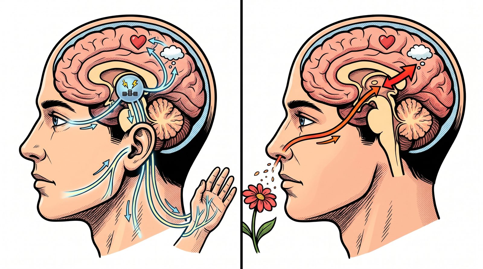
Left: information from the eyes, ears and skin passes through the thalamus first. Right: smell skips that stop and reaches emotion and memory regions directly. It’s also why marketers love scent. Hotel lobbies, shops, even the “new car smell” of some brands use carefully chosen fragrances. But measuring what a smell actually makes people feel is not easy. The answer to “did you like this smell?” is often only a small part of the experience.
Our Journey
Since 2022, our lab has run a series of studies on smell and EEG. With each one, the questions grew a little:
- Can we tell from EEG that a smell was presented? In our first studies, we tried to separate moments with and without an odour from brain signals alone. We saw this as a first step towards neuromarketing applications (SIU 2022, TIPTEKNO 2022).
- Which features capture that difference best? Next, we compared features drawn from different sides of the signal, such as time, frequency and complexity, and tried classic machine learning side by side with deep learning (TIPTEKNO 2024, Electrica 2024).
- What does a smell make us feel? In our latest studies we went a step further and tried to classify emotional responses to several different odours. One way was to turn EEG into a colourful heat map of the head seen from above, and analyse it with the convolutional neural networks we described in our CNN post (TIPTEKNO 2025).
In other words, we moved from “is there a smell?” towards “how does this smell feel?”.
Why Does It Matter?
Smell shows up everywhere, from product design to the experience of a space, and even in health, where tracking loss of smell matters. Being able to measure the emotional response to a smell, independently of what people say, gives all of these fields a new tool.
Burak Akbuğday, Sude Pehlivan Akbuğday, Dr. Faezeh Yeganli, Dr. Rıza Sadıkzade and Prof. Dr. Aydın Akan worked together on these studies. You’ll find the full list on our conferences page.
References
- The olfactory system as the gateway to the neural correlates of consciousness (2014). Frontiers in Psychology, 4, 1011. DOI: 10.3389/fpsyg.2013.01011
- Pehlivan, S., Akbuğday, B., Akan, A., Sadıkzade, R. (2022). Detection of Olfactory Stimulus from EEG Signals for Neuromarketing Applications. IEEE SIU. DOI: 10.1109/siu55565.2022.9864841
- Akbuğday, B., Akan, A., Pehlivan, S., Sadıkzade, R. (2022). An Assessment of Linear and Nonlinear Features for Detecting Olfactory Stimulus in EEG. IEEE TIPTEKNO. DOI: 10.1109/tiptekno56568.2022.9960190
- Pehlivan Akbuğday, S., Akbuğday, B., Yeganli, F., Akan, A., Sadıkzade, R. (2024). Decoding Olfactory EEG Signals Using Multi-Domain Features and Machine Learning. IEEE TIPTEKNO. DOI: 10.1109/tiptekno63488.2024.10755366
- Akbuğday, B., Pehlivan Akbuğday, S., Sadıkzade, R., Akan, A., Unal, S. (2024). Detection of Olfactory Stimulus in Electroencephalogram Signals Using Machine and Deep Learning Methods. Electrica. DOI: 10.5152/electrica.2024.23111
- Bozbas, O. A., Akbuğday, B., Akan, A., Pehlivan Akbuğday, S. (2025). Classification of Emotions Under Multiple Olfactory Stimuli Using EEG Signals and Machine Learning. IEEE TIPTEKNO. DOI: 10.1109/tiptekno68206.2025.11270194
- Yeganli, F., Akan, A., Sadıkzade, R. (2025). Olfactory Emotion Recognition Using EEG Spectral Topographic Heatmaps and CNNs. IEEE TIPTEKNO. DOI: 10.1109/tiptekno68206.2025.11270101
Can One Word On The Label Change How A Drink Tastes?
Does knowing what's in a drink change how we taste it? In the study we presented at IEEE CoDIT 2026, we asked participants, and we also looked at their brains.
There are two bottles of juice on the supermarket shelf. One label says “natural preservative”, the other names a chemical preservative. The ingredients are almost identical. Would they taste the same to you?

The same juice, two different labels. What we read on the label shapes how we imagine the drink, and how it tastes. Most of us would say “of course”. But taste doesn’t only happen on the tongue. What we think we’re eating or drinking also shapes how it tastes. That’s exactly what we wanted to find out in this study.
What Did We Do?
Participants tasted drinks containing different preservatives, and we varied the information they were given about the drinks beforehand. After each tasting, participants rated the drink. Meanwhile, we recorded their EEG with a 32-channel, water-based electrode headset.
That let us see two things side by side: what participants said, and what their brains did.
What Did We Find?
Both the type of preservative and the information given beforehand affected how participants rated the taste. In other words, knowing what was on the label changed how the drink was perceived.
On the EEG side, we saw two clear differences between the moments participants liked and disliked a drink: in gamma activity over the forehead, and in beta activity over the upper back of the head. We explained what these rhythms are in our EEG post.
Why Does It Matter?
Food labels don’t just inform; they shape the experience. Being able to show this with brain signals, alongside survey answers, helps us better understand what consumers mean when they say “I like it” or “I don’t”.
We presented the study at the 12th IEEE CoDIT conference in Bari, Italy, in July 2026. You’ll find the full reference on our publications page.
References
- Tunakan, B. İ., Akan, A., Taskin, Y., Turhan, K. N. (2026). Analysis of Human Emotions for Different Taste Stimuli Using EEG Signals. IEEE CoDIT. DOI: 10.1109/codit70676.2026.11630919
Neuromarketing, Or Listening To What Surveys Can't Tell You
We can ask people whether they like a product. But their answer isn't always the whole story of what they feel. Neuromarketing looks into that gap.
Picture yourself in a supermarket. Why did you pick one of the two shampoos on the shelf? Asked, you’d probably say “it smells nice” or “the price was right”. Yet some of what shaped your choice, the colour of the bottle, a familiar logo, your last experience with the brand, had already done its work before you noticed.
Traditional market research asks people: surveys, focus groups, interviews. These are valuable, but they have a weakness. People can’t always put what they feel into words, and sometimes they’d rather not. Neuromarketing tries to fill that gap by looking at brain and body signals at the moment a decision is made.
What Do We Measure?
- EEG: the brain’s electrical activity, recorded through electrodes on the scalp. It shows how the brain reacts within milliseconds to an advert or a logo.
- Galvanic skin response (GSR): when we get excited, our palms sweat ever so slightly. That tiny change is a marker of emotional arousal.
- Eye tracking: where the eye goes first on a package or a web page, and how long it lingers.
What Can’t We Measure?
Neuromarketing is not mind reading. EEG won’t tell you “this person will buy the product tomorrow”. What it can do, by averaging across many participants, is support comparative findings such as “this package triggers a stronger emotional response than that one”. A good study reads brain signals together with survey answers. Neither replaces the other.
In Our Lab
These are the questions we work on. With EEG, we study how sustainable packaging affects consumer behaviour, how information about preservatives in a drink changes the way it tastes, and what trust in a brand looks like in the brain. We’ll tell the story of each study in upcoming posts.
One last note: these studies run with ethics committee approval and the voluntary consent of every participant. The goal is not to steer people, but to understand what happens while they decide.
References
- Ariely, D., Berns, G. S. (2010). Neuromarketing: the hope and hype of neuroimaging in business. Nature Reviews Neuroscience, 11(4), 284–292. DOI: 10.1038/nrn2795
- Kilic, E. O., Akbuğday, B., Akan, A., Sadıkzade, R. (2026). Investigating the Effect of Sustainable Product Packaging on Consumer Behavior Using EEG Signals. IEEE CoDIT. DOI: 10.1109/codit70676.2026.11630728
- Tunakan, B. İ., Akan, A., Taskin, Y., Turhan, K. N. (2026). Analysis of Human Emotions for Different Taste Stimuli Using EEG Signals. IEEE CoDIT. DOI: 10.1109/codit70676.2026.11630919
- Pehlivan, S., Akbuğday, B., Akan, A., Sadıkzade, R. (2022). Detection of Olfactory Stimulus from EEG Signals for Neuromarketing Applications. IEEE SIU. DOI: 10.1109/siu55565.2022.9864841
A Flashlight Against Your Finger, What Does fNIRS Measure?
Looking into the brain with light sounds like science fiction. Yet fNIRS rests on the same idea as the red glow of a flashlight pressed against your finger in the dark.
In a dark room, press a flashlight against your fingertip. Your finger glows red. Some of the light makes it through skin, bone and blood and comes out the other side. The pulse oximeter clipped onto patients’ fingers in hospitals relies on this simple observation: it measures oxygen in the blood by looking at the light that passes through.

Light passes through skin, bone and blood and comes out the other side. How Does fNIRS Do It?
fNIRS (functional near-infrared spectroscopy) applies the same idea to the head. We place small light sources on the scalp, with light detectors a few centimetres away. Light from the source scatters through the tissue, some of it reaches the surface of the brain, turns back and arrives at the detector. By looking at how much of the light was lost on the way, we learn what is happening in the blood of that region.
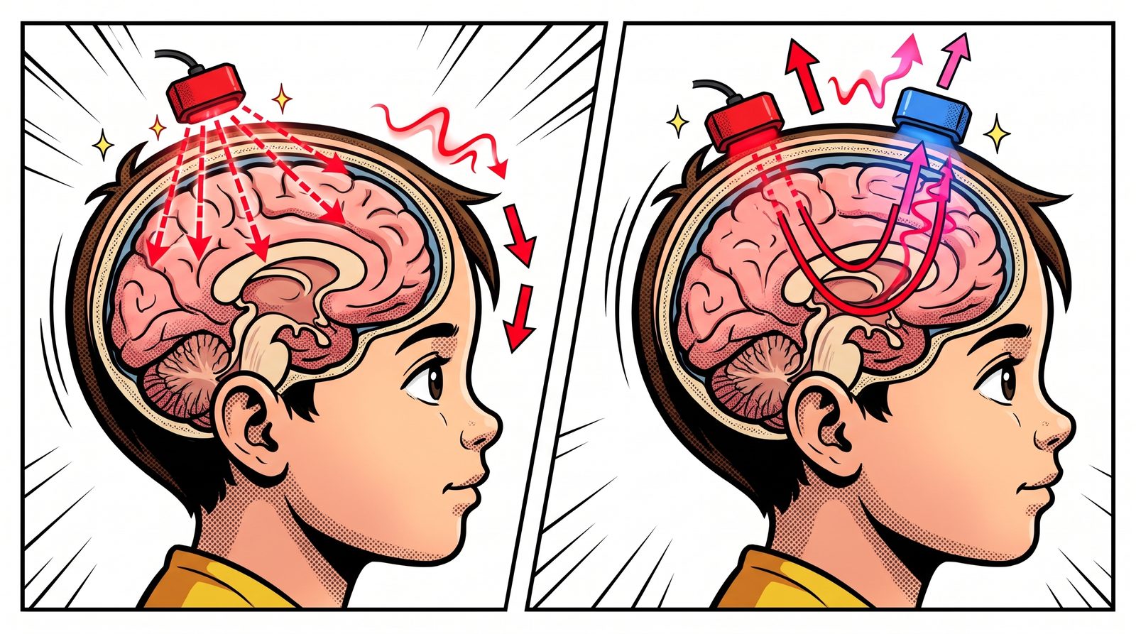
Left: light from the source scatters through the tissue. Right: part of it follows a curved path back to the detector (blue). Why Near-infrared?
Most visible light is absorbed as soon as it enters tissue. But for near-infrared light, roughly 700–1000 nanometres, biological tissue is surprisingly “transparent”. Frans Jöbsis noticed this “optical window” in 1977 and showed that light could cross the skull and reveal oxygen changes in the brain.
What makes this window useful is haemoglobin. Oxygen-carrying haemoglobin (HbO) and haemoglobin that has released its oxygen (HbR) absorb light differently at different wavelengths. By measuring at two wavelengths, we can work out the change in each of them separately.
A Working Region Asks For Blood
The brain has no real energy storage. When a region gets busy, fresh oxygenated blood is rushed there. This is called neurovascular coupling. Think of a city council adding extra buses to a neighbourhood at rush hour: when the crowd grows, the service grows too, often a bit more than needed.
As a result, oxygenated haemoglobin rises and deoxygenated haemoglobin falls in the active region. fNIRS picks up this opposite movement. So fNIRS doesn’t listen to neurons directly; it tracks the blood the neurons “ordered”.
A Banana-shaped Path
Light doesn’t travel from source to detector in a straight line. It scatters through the tissue along a curved, banana-shaped path. The farther apart the source and detector, the deeper the banana goes, but the less light comes back. In practice, a distance of about 3 centimetres in adults reaches the outer surface of the brain, the top few millimetres of the cortex. Deeper structures are out of fNIRS’s reach.
What Does The Output Look Like?
Each source–detector pair forms a channel. Labels like S1-D1 in the figure show which source is paired with which detector. Each channel gives us two curves over time: the change in oxygenated and in deoxygenated haemoglobin.
If we average these curves over a time window during the task and compare them with rest, we get a colour map over the head. Red areas are where oxygenated haemoglobin rose clearly during the task, the regions “ordering” more blood. Blue areas show no rise, or a drop.
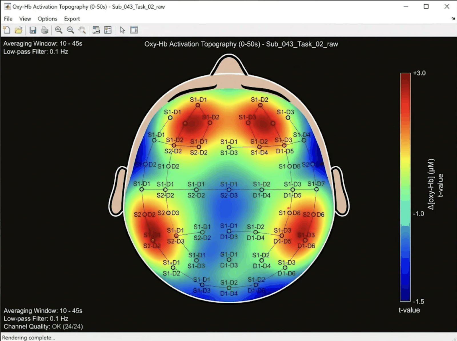
An illustrative fNIRS output: the distribution of oxygenated haemoglobin change over the head during a task. Compared With EEG
EEG listens to the roar from the stadium: it catches electrical activity within milliseconds but struggles to say exactly where the sound comes from. fNIRS watches the bus traffic heading to the stadium: changes in blood flow take a few seconds to show up, but which area is getting “crowded” is clearer.
That’s why the two are complementary, not rivals. Many studies use EEG and fNIRS together in the same cap: one answers “when” better, the other “where”.
Strengths And Weaknesses
Pros:
- Portable and silent. Nobody has to lie inside a tube; recordings can be made at a desk, while walking or while shopping.
- More tolerant of movement than fMRI, and much cheaper.
- Easy to use with babies and children.
Cons:
- It only sees the surface of the brain.
- Light passes through the scalp first, so blood flow in the skin leaks into the signal. Extra short-distance channels and signal processing are used to remove it.
- Dark, thick hair can block the light, and placing the optodes takes patience.
fNIRS In The Lab
The first functional fNIRS measurements in the human brain were made in 1992. Since then the field has moved from single-channel devices to wireless systems that cover the whole head. In our lab we are working on an improved whole-head fNIRS system that can run artificial intelligence on the device itself. For the latest on this work, see our TÜSEB news.
References
- Jöbsis, F. F. (1977). Noninvasive, infrared monitoring of cerebral and myocardial oxygen sufficiency and circulatory parameters. Science, 198(4323), 1264–1267. doi:10.1126/science.929199
- Ferrari, M., Quaresima, V. (2012). A brief review on the history of human functional near-infrared spectroscopy (fNIRS) development and fields of application. NeuroImage, 63(2), 921–935. doi:10.1016/j.neuroimage.2012.03.049
The Transformer, A Meeting Where Everyone Can Look At Everyone
The Transformer, the architecture behind language models like ChatGPT, doesn't read a sentence word by word. It looks at all the words at once and decides which ones relate to which.
Read this sentence: “The cat knocked over the milk bowl because it was hungry.” What was “it”? The cat, of course. Now this one: “The cat knocked over the milk bowl because it was on the edge of the table.” This time “it” is the bowl. You read the same word in both sentences, but to decide what it means, you have to look at the rest of the sentence.
That’s the core idea behind the Transformer architecture, introduced in 2017: attention.
A Meeting Instead Of Reading In Order
The LSTM we described in the previous post reads a sentence left to right, word by word, noting what it sees in a notebook along the way. It works, but it’s slow, and as the sentence grows longer the early information can still fade.
The Transformer treats the sentence like a meeting table instead. Each word is a person at the table, and everyone can look at everyone at once. The word “it” asks the table: “Who decides my meaning the most?”. In the first sentence, “hungry” and “cat” answer loudest. In the second, “edge of the table” and “milk bowl”.
That’s how each word decides how much attention to pay to the others. The process is called self-attention.
Why Does It Work So Well?
It has two big advantages. First, it easily captures relationships between distant words. A word at the start of the sentence can “talk” directly to one at the end. Second, because it looks at everything at once, it trains very fast on modern computers. That’s what made large language models, trained on enormous amounts of text, possible.
By the way, the people at the table don’t have to be words. They can be patches of an image, notes in a piece of music, or consecutive time windows of an EEG signal.
Transformers And EEG
In EEG, relationships between different electrodes and different moments in time matter a lot. For example, whether a change over the forehead is linked to a change at the back of the head a few hundred milliseconds later. The Transformer’s “everyone can look at everyone” design is a natural tool for learning such distant relationships. Most of the large “foundation models” built in recent years to understand EEG are based on this architecture.
References
- Vaswani, A. et al. (2017). Attention Is All You Need. NeurIPS. arXiv:1706.03762
LSTM, The Network That Knows What To Remember And What To Forget
When you watch a series, you keep earlier episodes in mind, but not every detail. LSTMs handle sequential data the same way.
Imagine you’re watching a long TV series. When a character in the new episode says “You were the one who told me”, you need to remember what happened three episodes ago to make sense of the scene. On the other hand, you don’t need to remember the colour of someone’s jacket in that episode. Your brain picks what matters, keeps it, and lets the rest go.
Sequential data, such as words in a sentence or EEG measurements arriving one after another in time, works the same way. To understand the current step, you need to know what came before. LSTM networks (Long Short-Term Memory) were designed for this.
A Notebook And Three Gates
Think of an LSTM as a viewer holding a notebook. With every new scene, it makes three decisions about that notebook:
- Forget gate: Which notes no longer matter? The jacket colour can go.
- Input gate: What happened in this scene that’s worth writing down? The argument between two characters should be noted.
- Output gate: Which notes should I look at to understand the current scene?
These “gates” are really dials. During training, the network learns for itself when and how far to open or close each one.
Why Does It Matter?
Simpler sequential networks before LSTM had a big problem: forgetfulness. Information from just a few steps back faded quickly. The notebook idea let important information survive for a long time. That’s why LSTMs were widely used for years in speech recognition, translation and weather forecasting.
LSTMs And EEG
EEG is a long time series with hundreds of measurements per second. To catch an emotional reaction or the moment attention slips, you can’t look at a single instant; you need to see how the signal changes over time. LSTMs can learn such patterns by reading the signal step by step and “remembering” the important changes.
In the next post, we’ll look at the Transformer architecture, which looks at the whole sequence at once instead of reading it in order.
References
- Hochreiter, S., Schmidhuber, J. (1997). Long Short-Term Memory. Neural Computation, 9(8), 1735–1780. DOI: 10.1162/neco.1997.9.8.1735
How Does A CNN Work? Looking At A Painting With A Torch
Convolutional neural networks don't take in an image all at once. They look at it piece by piece, like studying a painting in a dark room with a small torch.
There’s a painting on the wall of a dark room, and you’re holding a small torch. You can’t see the whole painting at once. You start in the top-left corner and sweep the beam slowly across. Each time a small patch lights up: a line here, a curve there, a change of colour further along. In the end you put the pieces together in your head and say: “it’s a portrait.”
Convolutional neural networks (CNNs) look at images in exactly this way. A 1998 paper by LeCun and colleagues was a milestone in shaping the idea as we know it today.
Small Templates
Instead of a torch, a CNN has small templates. Each template specialises in finding one thing. One looks for vertical lines, another for horizontal ones, another for a particular colour change. The network slides each template across the whole image and notes, “is what I’m looking for here, and how much of it?”. That sliding is called convolution.
The nice part is that no one designs these templates by hand. As the network sees thousands of examples, it learns for itself which templates are useful.
Meaning, Layer By Layer
Templates in the first layer find very simple things: edges, corners. The second layer combines what the first found. A few edges side by side make the shape of an eye. Higher layers combine those shapes: if two eyes, a nose and a mouth appear together, there’s probably a face.
In between there’s a summarising step (pooling). Think of it as stepping back from the painting. Some detail is lost, but the fact that “there’s an eye here” remains. That way the network doesn’t get hung up on the exact pixel where the eye sits.
So What Does This Have To Do With EEG?
EEG isn’t an image; it’s a signal that changes over time. But we can turn it into a colourful map showing which frequencies grow stronger or weaker over time: a time–frequency image. That map is a picture, and CNNs are very good at spotting patterns in it, such as those typical of an emotional state or a disease. Many studies in our lab, for example on epilepsy, dementia and liking, build on exactly this idea.
In the next post, we’ll look at LSTMs, which process data that arrives in sequence by “remembering” what came before.
References
- LeCun, Y., Bottou, L., Bengio, Y., Haffner, P. (1998). Gradient-based learning applied to document recognition. Proceedings of the IEEE, 86(11), 2278–2324. DOI: 10.1109/5.726791
- Epileptic EEG Classification by Using Time-Frequency Images for Deep Learning (2021). International Journal of Neural Systems. DOI: 10.1142/s012906572150026x
- Classification of Dementia EEG Signals by Using Time-Frequency Images for Deep Learning (2023). IEEE ASYU. DOI: 10.1109/asyu58738.2023.10296777
- Liking State Estimation Using Time-Frequency Image Representation of EEG Signals (2025). IEEE SIU. DOI: 10.1109/siu66497.2025.11112167
Our Blog Is Live
We will use short posts here to share what we do in the lab, the behind-the-scenes of our experiments and what we learn along the way.
Our publications describe the results of our work, but rarely the path that led there. This blog is where we want to share that path: how an experiment was designed, the problems we ran into while recording, and why an analysis method did or didn’t work.
Posts will be short and will come from different members of the team. If you’d like to ask a question or work with us, you can always get in touch.

No posts under this topic yet.